Chapter 5: Correlation
Correlation is an inferential statistical test. That is, we use it to ask a particular kind of research question in relation to some data and the output tells us something about the extent to which we can expect our observations to generalize is we collected more data.
Correlations are used when we want to investigate the relation between two continuous variables. Basically, we can observe three kinds of relations (to varies degree):
1) A positive relation: this means that whenever we observe a higher value in one variable it will correspond to a higher value in the other variable. An example could be that vocabulary size (variable 1) is systematically associated with the age of children (variable 2) meaning that the older the child the bigger the vocabulary.
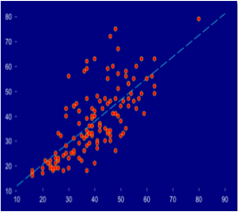
Figure 1: scatter plot illustrating a positive relation between two continuous variables
2) A negative relation: when we observe a higher value in one variable it corresponds to a lower value in the other variable. An example could be the relationship between training and reaction time in a task. The more training, the shorter the reaction time.
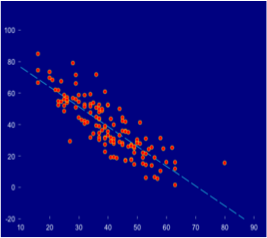
Figure 2: scatter plot illustrating a negative relation between two continuous variables
3) No relation: there is no systematic relation between the scores so an increment in one variable can be followed both by positive and negative or no tendency in the other variable.
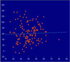
Figure 3: scatter plot illustrating a case of no relation between two continuous variables
The output of a correlation analysis
A correlation analysis returns two outputs: a correlation coefficient and a p-value. From the correlation coefficient we can also easily calculate the coefficient of determination, R2, which
The correlation coefficient, r
The correlation coefficient, often denoted r, is an expression of the effect size, that is, the strength of the relation between the variables. It is a value between -1 and 1, where -1 = a perfect negative relation, 0 = no relationship and 1 = a perfect positive relationship. A more or less generally agreed upon interpretation of the effect size is given below:
| r | Interpretation of effect size |
|---|---|
| 0 | no relationship |
| ±.1 | small effect |
| ±.3 | medium effect |
| ±.5 | large effect |
Figure 4: Interpretation of the effects size of correlation coefficients
The p-value
The p-value is the probability that the NULL-hypothesis is true given the data. In most cases, we don't want the NULL hypothesis to be true. That would mean that there is no relationship between our variables. Often we are testing the hypothesis that there in fact is a relationship, that is, we want to prove the NULL hypothesis wrong.
We can reject the NULL hypothesis (and thus support your hypothesis) if the p-value is low, i.e. if the probability of the NULL hypothesis being true is low.
By mere convention in the field it has been decided to set a fixed threshold at p = .05. That means that if the p-value if below .05 we are safe to reject the NULL hypothesis, which effectively mean that we confirm our (positive) hypothesis: there is a significant relationship between our variables.
The p-value is generally interpreted as an expression of the probability that our results would generalize if we went and collected more data.
Assumptions for correlation
The standard correlation procedure is called Pearson's correlation coefficient. We use this most of the time. However, since it is a parametric test, it rests on the assumption of normality and the assumption of homogeneity of variance.
Testing normality
Let's imagine that we wanted to test if there is a relation between people's shoe sizes and there ability to their hold breath. We got the impression that there could be a positive relationship from the scatter plot we made in the previous chapter.
In order to test the relationship with a Pearson's correlation analysis, both variables, in this case shoe sizes and holding breath times, need to be normally distributed. We covered different ways to tests for normality in the previous chapter. While visual judgments (based on histograms and/or q-q plots) often are the best choice, there are also numeric, statistical tests that can support our judgments, such as the Shapiro-Wilk test. If the test is significant (p < .05), our variable is not normally distributed (Notice that the Shapiro-Wilk test is built into the stat.desc() function introduced in the previous chapter).
In order to test for the assumption of normality in the case of shoe sizes and holding breath, we need first to import a data set (if we have not already done so).
  # set working directory
  setwd("~/path to your data/")

  # Import data
  data = read.delim('SampleDataSet.txt')
Then we can use the R command shapiro.test() to test if our variables of interest are normally distributed.
  # test if shoe size data are normally distributed
  shapiro.test(data$Shoe_size)

  # test if shoe size data are normally distributed
  shapiro.test(data$Hold_breath)
Let's have a look at the out of the analysis:

Figure 4: Output of the Shapiro-Wilk test of the shoe size data

Figure 5: Output of the Shapiro-Wilk test of the holding breath data
For the shoe size data, we notice that the p-value is above the .05 threshold which means that the data is normally distributed. However, for the holding breath data the p-value is lower than the threshold indicating the that data is not normally distributed.
Testing homogeneity of variance
Also, correlations rest on the assumption of homogeneity of variance. This means that the variance of one variable should be stable across all levels of the other variable. We can test for this assumption using Levene's test. If the test is significant (p < .05), the variances are unlikely to have occurred from a population with equal variances, that is, the data violate the assumptions of homogeneity of variance.
The R function levenTest() is part of the carpackage. If you have not already installed this package you will need to do this first.
  # install the package 'car'
  install.packages('car')
Now we can proceed and test our variables of interest.
  # load the car module
  library(car)

  # run the Levene's test
  leveneTest(data$Shoe_size, data$Hold_breath)
Let's have a look at the output of the test:

Figure 6: Output of the Levene's test for homogeneity of variance between shoe size and holding breath
We observe that the p-value is above the significance threshold and we can conclude that our variables conform to the assumptions of homogeneity of variance.
Pearson's Correlation Coefficient
The standard parametric correlation test is Pearson's correlation. If our data conform to the assumptions, we use this test (if not, see Spearson's rho below). There are several commands that we can use to run a Pearson's correlation in R. However, here we will introduce only one, the cor.test().
The syntax of this function is really simple. We just have to insert the two variables for which we predict some systematic relation separated by a comma. In the example from above, those were shoe sizes and seconds of holding breath.
  # testing the relation between shoe size and holding breath
  cor.test(data$Shoe_size, data$Hold_breath)
Let's have a look at the output:
 Figure 7: Output of the Pearson's correlation of shoe sizes and ability to hold breath
The output of the analysis gives us (among other things) a correlation coefficient (the cor = 0.46), degrees of freedom (df = 27), and a p-value (p-value = 0.012). We notice that the correlation coefficient is r = .46. This corresponds to a "medium" effect size. We also observe that the p-value is below the threshold of .05 which means that the correlation coefficient is significantly different from zero, or in simple terms: that the correlation is significant.
In addition, we can calculate the r-squared, R2, simply by multiplying the rho value with itself.
  # calculate the r-squared
  0.4590705 ^ 2
This value is often called the coefficient of determination and is - in the case of correlation - interpreted as the amount of shared variance between the variables.
However, remember that one of the variables, the holding breath data, was actually not normally distributed, and therefore the result of the parametric Pearson's Correlation is probably unreliable. The solution is either to try and do a log-transform of both variables and test normality again or to do a non-parametric correlation test such as Spearman's rho (see below).
Spearman's ranked correlation coefficient
This is the option to use if your data violate the assumptions of parametric tests. The Spearman's rank correlation coefficient (or Spearman's rho) resample the data as ranked (rather than continuous). This solves some of the issues with influential outliers or skew. The procedure is the same as with Pearson's correlation. We can use the cor.test() function in R and just specify that we want the 'spearman' method.
  # testing the relation between shoe size and holding breath
  cor.test(data$Shoe_size, data$Hold_breath, method = 'spearman')
Let's inspect the output (and compare it to the output of the Pearson's correlation):
 *Figure 8: Output of the Spearman's ranked correlation of shoe sizes and holding breath
We notice that the rho (which is the Spearman equivalent of the correlation coefficient, r) = .50. This is actually slightly higher than the Pearson's correlation coefficient and corresponds to a "large" effect size (this is not always the case). We also get a p-value, which again is lower than for the Pearson's correlation, suggesting higher level of significance. The Spearman method does not output the degrees of freedom (df), but for correlation this is always n - 2, i.e. number of observation minus two: in this case df = 27.
Again, we can also calculate the R2 following the procedures from the section above.
Reporting correlations
The APA (American Psychological Association) convention for reporting correlation is as follows:
Pearson's correlation
"The ability to hold breath (measured in time) significantly correlated with participants shoe size, r(27) = .45, p < .05, R2 = .21"
Spearman's ranked correlation (rho)
"The ability to hold breath (measured in time) significantly correlated with participants shoe size, rs(27) = .50, p < .01, R2 = .25"
Notice that in both cases we first report r (or rs), followed by degrees of freedom in brackets and then the correlation coefficient. After this we report the p-value and, optionally, the R2.
Often we will accompany the numeric report with a scatter plot with a regression line illustrating the result of the analysis (see previous chapter).