Chapter 100: Data (re)structure
It's time to start thinking about how we structure our data. Working around problems with data structure often takes up a large portion of the time it takes to run an analysis or complete an assignment.
You'll want to fill your programming toolbox with fast tools. For data analysis, the important thing is often how fast/easy it is for the programmer to work with, rather than how fast the computer can run the code once it's written.
It may be possible to rewrite your code base in C to make it 100 times faster. But if this takes 100 human hours it may not be worth it. Computers can chug away day and night. People cannot.
Lovelace, Robin, and Morgane Dumont. 2016. Spatial Microsimulation with R. CRC Press. Free online version at https://csgillespie.github.io/efficientR/introduction.html#what-is-efficiency
Tidy Data
The biggest waste of your time is inconsistent data structure. A good way to think about your data is the concept "tidy data".
Tidy data has:
- One variable per column
- One observation per row
- One value per cell
Sometimes what you call "a variable" or "an observation" may change depending on the context (your hypothesis). For instance, when analyzing the CHILDES corpus, which is a corpus of data from interviews with a mother and her child, we could compute the mean length of utterance (mlu) for both the mother and the child.
Q: Which of these formats are correct? What are the variables?
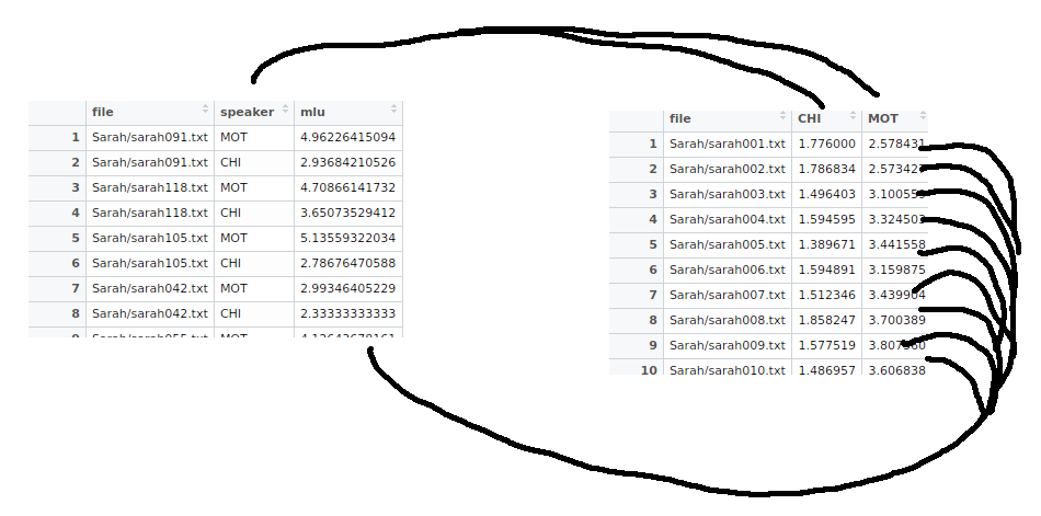 Figure 1: Tidy data. Two formats that could both be called tidy, depending on the context. The hand-drawn lines map data from one format to the other.
A: Well, that depends. If you think the mlu is a measure than you then want to take for each of the interaction partners (mother and child), you could structure it like I've done on the left. In this case, we have two observations per interview, and thus need two rows per file.
A: Or if you think mlu for the mother and child are qualitatively different measures, you could call them variables and store them like I've done on the right. Here, there's one observation (mlu of both) per interview, so one row per file.
Tidy functions
In the next few sections, we will go through some functions that try to tidy the data or operate on tidy data.
Common to them all is that they always take a data frame as the first argument, and return a data frame as the output. This consistency makes it easy to work with, since you'll always know what each function expects and returns (if not, use the built-in help, ie: ?gather).
Later you'll also see how tidy functions enable us to string operations together for easily readable code.
A lot of them come from the packages tidyr and dplyr
install.pacakges(c("tidyr", "dplyr))
library("tidyr")
library("dplyr")
gather() and spread()
Also called reshaping, or melting and casting, or converting between "wide" and "long" format. gather() and spread() are probably the data restructuring tools used most often in our kind of R programming.
To convert our dataframe from the format on the left to the one on the right in figure 1, we can spread() the key:value pair across columns. In our case, the key is the speaker column, and the values are in the mlu column, and there are only two different keys (MOT and CHI), so we get two columns out of it.
data_wide = spread(data_long, speaker, mlu)
This could be useful for functions that takes two vectors as input:
> cor(data_wide$MOT, data_wide$CHI)
[1] 0.635041
Or, to convert from the format on the right to the format on the left in figure 1, we can gather() as many columns as we'd like (in our case just the MOT and CHI columns) into a key column ("speaker") and a value column ("mlu")
data_long = gather(data_wide, "speaker", "mlu", CHI:MOT)
This format is often useful for model fitting
model1 <- lm(mlu ~ speaker, data_long)
or plotting with groups
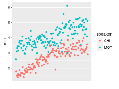
Figure 2: "long format" data created with gather() can be useful for plotting and modelling
mutate() and summarise()
Mutate adds new columns to an existing dataframe (one new value per row), and summarise returns just one summary statistic.
> mutate(data_wide, difference = MOT - CHI)
                file      CHI      MOT difference
1 Sarah/sarah001.txt 1.776000 2.578431  0.8024314
2 Sarah/sarah002.txt 1.786834 2.573427  0.7865927
3 Sarah/sarah003.txt 1.496403 3.100559  1.6041558
4 Sarah/sarah004.txt 1.594595 3.324503  1.7299087
5 Sarah/sarah005.txt 1.389671 3.441558  2.0518871
6 Sarah/sarah006.txt 1.594891 3.159875  1.5649841
> summarise(data_wide, mean_difference = mean(MOT - CHI))
  mean_difference
1        1.379489
The pipe %>%
Very often, you'll need to do more than one thing to your data. The pipe operator %>% is a handy way to string together operations in a humanly-readable way.
data_long %>%
  spread(speaker, mlu) %>%
  mutate(difference = MOT - CHI) %>%
  summarise(mean_difference = mean(difference))
What it does is that it sends the output from the previous code into the next code as the first argument to the function. That means that the code above is 100% equivalent to the code below, but much more readable. Notice also the intuitiveness of the order of operations (first spread, then mutate, then summarise):
summarise(
  mutate(
    spread(
      data_long, speaker, mlu),
    difference = MOT - CHI),
  mean_difference = mean(difference))
In either case, the results are the same:
  mean_difference
1        1.379489
group_by()
This is where these functions really start to shine. group_by() is a way to use the common "split-apply-combine" strategy in a way that's efficient for the programmer to think about. In the previous examples, summarise() only returned one value, but with a grouped dataframe, summarise() will return one value per group. mutate() still returns one value per row, but if you use aggregates (ie the mean), you will get the mean for each group separately:
data_long %>%
  group_by(file) %>%
  mutate(m = mean(mlu))
                 file speaker      mlu        m
1  Sarah/sarah001.txt     MOT 2.578431 2.177216
2  Sarah/sarah001.txt     CHI 1.776000 2.177216
3  Sarah/sarah002.txt     MOT 2.573427 2.180130
4  Sarah/sarah002.txt     CHI 1.786834 2.180130
5  Sarah/sarah003.txt     MOT 3.100559 2.298481
6  Sarah/sarah003.txt     CHI 1.496403 2.298481
In the example below, we calculate a mean and .95 confidence intervals manually for the mother and the child separately.
data_long %>%
  group_by(speaker) %>%

  summarise(
    m.mlu = mean(mlu),
    se = sqrt(sum((mlu - m.mlu)^2)/n()/(n() - 1)),
    Lower = m.mlu - se*1.96,
    Upper = m.mlu + se*1.96,
    conf.sig = ifelse(Lower > 0,"*", " ")) %>%

  ggplot(aes(speaker, ymin=Lower, y=m.mlu, ymax=Upper)) +
    geom_bar(stat="identity") +
    geom_errorbar(width=.3) +
    geom_text(aes(y = Upper + 0.1, label=conf.sig), size=8)
  speaker    m.mlu         se    Lower   Upper conf.sig
1     CHI 2.691630 0.05651519 2.580860 2.80240        *
2     MOT 4.071119 0.05616871 3.961028 4.18121        *
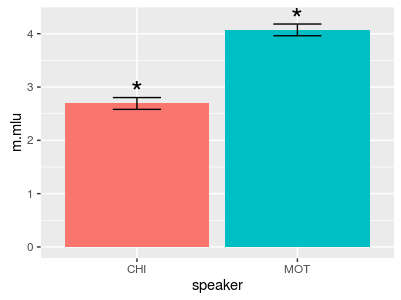
Figure 3: Using group_by(), we can calculate anything we want (in this case .95 confidence intervals) for each group
Combining data
We can combine data in many different ways.
We could have two almost identical dataframes (data from two participants) that we want to combine by adding the new data as new rows. This is done with bind_rows(data1,data2). If you don't have the information in the dataframe already, it can be helpful to add a column with the participant ID
bind_rows(mutate(data1, ID=1),
          mutate(data2, ID=2))
Another common way to join data is when you've got sepearate dataframes for separate types of information. For instance, you could have a data frame with multiple rows per participant (one for each observation), and another with some additional participant information that has just one row per participant. You can join these two dataframes by matching if you have common column that maps them (could be a name or an id).
left_join() keeps all the data from the first dataframe, and fills out new columns based on the second. At the end of this chapter, there's a link to a data wrangling cheat sheet that has really helpful illustrations for what the different kinds of joining operations do.
> head(data_long)
                file speaker      mlu
1 Sarah/sarah001.txt     MOT 2.578431
2 Sarah/sarah001.txt     CHI 1.776000
3 Sarah/sarah002.txt     MOT 2.573427
4 Sarah/sarah002.txt     CHI 1.786834
5 Sarah/sarah003.txt     MOT 3.100559
6 Sarah/sarah003.txt     CHI 1.496403
> head(extra_data)
                file hours_sunlight
1 Sarah/sarah001.txt              4
2 Sarah/sarah002.txt              3
3 Sarah/sarah003.txt              1
4 Sarah/sarah004.txt              5
5 Sarah/sarah005.txt              6
6 Sarah/sarah006.txt              4
> left_join(data_long, extra_info)
Joining, by = "file"
                  file speaker      mlu hours_sunlight
1   Sarah/sarah001.txt     MOT 2.578431              4
2   Sarah/sarah001.txt     CHI 1.776000              4
3   Sarah/sarah002.txt     MOT 2.573427              3
4   Sarah/sarah002.txt     CHI 1.786834              3
5   Sarah/sarah003.txt     MOT 3.100559              1
6   Sarah/sarah003.txt     CHI 1.496403              1
Use cases
- Fixing messy data from someone else's data collection
- Re-structuring data for a different level of analysis
- Run the same pre-processing on multiple columns
- Plotting data from multiple analyses in one plot
Additional materials
For a cheat sheet with all the functions and nice illustrations, have a look at the data wrangling cheat sheet from RStudio:
https://www.rstudio.com/wp-content/uploads/2015/02/data-wrangling-cheatsheet.pdf
A lot of these ideas are taken from Hadley Wickham's book "R for Data Science", which I (Malte) really recommend you go skim through if you want to get better at R
Sometimes tidy data is not the best